Thoughts On Over a Decade of Magnetic Resonance Fingerprinting
March 14, 2023
Back in January I had a wonderful dinner conversation with Efrat Shimron and Eddy Solomon about some of the history of Magnetic Resonance Fingerprinting (MRF) at the ISMRM Workshop on Data Sampling in Sedona, Arizona. There’s so much that our lab never published and both of them suggested that I write some of this up so that others could see how we got to MRF. We’ve had some health issues in my family so I’ve been a bit delayed in writing anything, but today marks the 10-year anniversary of our paper in Nature. This is by far one of the most important papers I’ve ever been a part of. We also got the news last week that Siemens got FDA approval for their MRF product, so the timing is probably right to get some thoughts down as the next crop of new researchers and clinicians start to use this method in clinical situations.
So based on my conversation with Efrat and Eddy, I thought I’d cover two topics that might be of interest for folks in our field: 1) Early history and how we got to MRF from compressed sensing and 2) What makes an acquisition MRF? We covered some of topic 1 at the ISMRM Workshop on MRF in 2017, but not everyone could attend, so I’ll retell some of that. In retrospect the links to compressed sensing probably weren’t clear in the Nature paper, largely because we had a very tight word limit, but it’s key to the origin story. Topic 2 has come up several times in the recent past, especially in the context of new papers and reviews, and I’ll do my best to show how we’ve defined MRF over the years. I’ll likely post this next week. But to start off… some history!
MRF From Compressed Sensing
All of us who contributed to MRF have a different perspective. But for me, the story of MRF actually starts sometime around 2003. I was still living in Würzburg Germany and we had just gotten the product GRAPPA recon up and running on the Siemens platform. We were also putting in a huge effort to build 32 channel coils for the first time. At the same time, I had been working with Peter Schmitt to try to understand relaxation effects in balanced SSFP(bSSFP)/TrueFISP. Klaus Scheffler had published a paper using IR-bSSFP for T1 mapping. But when we tried it in the brain, we saw that it could be heavily influenced by T2. I had a conversation with Klaus about this at the time, and he told me that they had only been using short windows to read out the signal, and so they weren’t that sensitive to T2. We set out to try to understand this and eventually published two of my favorite papers: one on IR-bSSFP for T1 and T2 mapping and one on a simplified geometric description of bSSFP which we actually did first, but published second. That paper was a masterwork by Peter who derived the eigenstates of off-resonant bSSFP on paper over a weekend. That work still amazes me! Without a doubt one of my favorite papers! At the same time, we were looking at ways to modify the transient state of a bSSFP acquisition in order to highlight different properties of the transient. Again a favorite paper that we published much later than when we did the work was the TOSSI method to generate almost purely T2-weighted decays from bSSFP acquisitions.
The timing was perfect for this work too as Vikas Gulani had come to the lab on a research year during his radiology residency and immediately saw the importance of quantitative imaging in the clinical world. We published a nice paper on using IR-TrueFISP for T1, T2 and M0 quantification but when we tried this more broadly in the clinic, we realized that it was too slow for widespread adoption and was sensitive to things we didn’t want, like B1+ and slice profile. Both Vikas and I would end up moving to Cleveland, Ohio and would eventually recruit Dan Ma and Nicole Seiberlich to work on this problem using various methods.

But in retrospect the real change in our trajectory had happened back in 2004 but we just didn’t know it yet. At an MR Angio Club meeting, Chuck Mistretta handed me a preprint of “Robust uncertainty principles: exact signal reconstruction from highly incomplete frequency information” by Emmanuel Candes, Justin Romberg and Terry Tao, one of the papers that would form the bedrock of what we now know as compressed sensing. It was pages of dense math that I couldn’t grasp all at once, but when he handed me the paper, Chuck (paraphrasing) basically said “You may not need to do all of that work on those 32 channel coils. This paper says you can get the same results just with a different reconstruction.” Chuck would go on to develop one of the first modern MRI methods to exploit sparsity of angio sequences, HYPR, and defined the term “post-Nyquist imaging”, which I still like very much. But I honestly looked at the paper initially and said “Bullshit. There’s no way that’s going to work in practice.” But I had a long flight back to Germany, and spent most of that flight trying to disprove the paper, which I obviously couldn’t do. But I also couldn’t get good images either! It took until Miki Lustig published the first compressed sensing MRI paper that I really saw good compressed sensing MRI images.
But if you look at the publication history of our lab, we’ve largely stayed away from compressed sensing for our clinical work. Especially in the early days, we saw too many incidents of reconstructions that would hide important anatomical features or would have strange noise behavior, etc. and in our integrated clinical lab, we just couldn’t see a way to fix these intolerable and seemingly random errors. But on the other hand, the math said that there had to be something there. I actually spent several hours a week for at least six months reading Emmanuel Candes’s abstract “Compressive Sampling” which he wrote for the Proceedings of the International Congress of Mathematicians, Madrid, Spain, 2006 trying to understand every detail. This is honestly one of the best explainers of the concept that I’ve found. Everyone in our field should at least understand the first four pages of this paper. Just the simple description of how you can go from Nyquist to Papulous to compressed sensing is genius. Seriously just go read it! (The other great one is Terry Tao’s blog post explaining a single pixel camera).
At the end of the day, my conclusion of compressed sensing at that point was that one always had to make an assumption that was fundamentally wrong. All of the formulations that I was aware of were balancing a data consistency constraint (which you could do perfectly) with some assumption about the object, like sparsity in wavelets, or total variation, none of which could be true in a real life situation. You could get close, but the error from those terms could never be zero in real life. It retrospect, it’s clear that you can make a wrong-ish spatial assumption that can still decrease your overall error to the point where you can dramatically improve image quality (like Miki’s fantastic work with Shreyas Vasanawala in pediatric patients like this paper), but I personally wanted to make a right assumption that would do the same thing. So I spent the first years of compressed sensing thinking about what kind of constraint could always be correct and would reduce image error in accelerated imaging. But as far as I could tell, you can’t do this in a spatial domain unless you already know what the object looks like.
So it was around this time, that we started thinking about other domains, and we very quickly realized that a domain where you could make an exact constraint was the time domain, and we already had years of experience trying to do quantitative mapping. We had tried several compressed-sensing approaches, but none of them were really great, and the reconstruction time was through the roof. But the real breakthrough in our thinking happened when Mariya Doneva and colleagues published their groundbreaking work in this area “Compressed sensing reconstruction for magnetic resonance parameter mapping”. In my mind, this was the first time that anyone had used a dictionary of timecourses for reconstruction of quantitative MRI data. But in this case, Mariya was calculating dictionaries and then calculating the match across the components of the SVD of the full dictionary. But the opportunity was there now for a perfect constraint. If we could calculate a dense dictionary that could span the whole range of relaxation values that one would expect, you could potentially get the perfect constraint, maybe even down to a match with just one dictionary entry, which would correspond to perfect sparsity in a compressed sensing context… one dictionary entry contributing with all others having a zero contribution. This was what we were looking for.
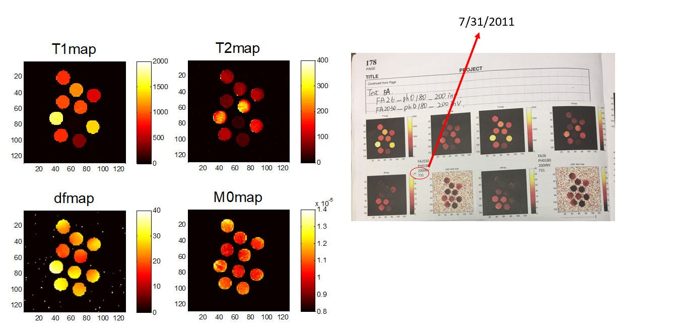
At the same time, we were back to thinking about the acquisition. You only have to do a few IR experiments to realize how inefficient they can be. If you’re scanning in the brain you have to scan for many seconds to get an accurate map of fluid, but you have things like fat and white matter which have relaxed many times over by the time you finish the acquisition. So we were back to asking whether there could be a better acquisition. This is when the hours of reading Candes’s paper paid off—let’s treat the Bloch equations like a system matrix that we’re trying to solve. Without worrying too much about details, one of the core tenets of compressed sensing is that you can get really close to the optimal answer by just probing the problem with random projections. So that’s what we tried—let’s do random flip angles and TRs and see what comes out. And very quickly we saw that we could get much higher efficiency than conventional IR-bSSFP imaging and that it didn’t really matter what we did. (We also saw that purely random sucks, but smoothed random-like sequences were all pretty good.) Combined with the ideally-sparse dictionary reconstructions, we had something that was really working… at least on a computer. Dan and I have gone back and found our original emails about this from October of 2010. The first 1D phantom experiments didn’t work until January of 2011. The first 2D phantom results were July 31, 2011. And then she ended up presenting the first in vivo results at the 2012 ISMRM.

I won’t spend a lot of time on this, but writing a paper for Nature is a trip! We thought we had done a reasonable job on the first submission, but the first review came back about 2x the length of the original submission! But to be honest, I still think it’s one of the best reviews I’ve ever gotten. The reviewers made so many excellent points that it truly improved the paper. We had a really short time to turn around the revision and I think Dan and I almost lived in the lab that month, but it was obviously worth it! Right now, the Nature metrics say, “This article is in the 99th percentile (ranked 104th) of the 197,229 tracked articles of a similar age in all journals and the 98th percentile (ranked 11th) of the 994 tracked articles of a similar age in Nature.” It’s been a real honor to be a part of this journey and I’m so happy that we’ve now been able to take this concept from its initial conception all the way through to clinical implementation.


I’ll try to post my 2 cents on what makes an acquisition MRF as well as some clinical hints in the coming weeks. But for today, in addition to some early MRF images, Dan also reminded me that we also just passed the 10 year anniversary of the first Music MRF scan. Here’s the first video of that that Dan sent me on Feb 14, 2013. Hope you enjoy!
Take care!!
--Mark


